Introduction
For this laboratory exercise, you will be asked to build a Digital Differential Analyzer (DDA) in Verilog that integrates the Lorenz system. The Lorenz system generates (arguably) one of the most famous and beautiful structures in mathematics: the "butterfly curve" (from which the "butterfly effect" gets its name). For certain parameter values and initial conditions, the solutions for the Lorenz system are chaotic. That is to say, they are deterministic yet unpredictable. The solutions are so sensitive to initial conditions that, after sufficient time, it is no longer possible to determine the path that the system will take without running a simulation. Meditate on the notion of "deterministic yet unpredictable" for long enough and you may end up questioning things like your own free will. But I digress.
The DDA circuit that you build will be controlled by the HPS. Controlling the DDA involves clocking it and setting initial conditions/parameter values. You will build a system that allows for you to play with the Lorenz system. The VGA screen will display all three projections of the 3D curve, and your user interface will support speeding up/slowing down animation, pausing/resuming animation, clearing the screen, dynamically changing parameters, and resetting with a new set of user-specified initial conditions.
Finally, you will implement three Direct Digital Synthesis synthesizers in Verilog that independently generate three tones from a speaker. Those tones will be functions of the x, y, and z state variable values, and will allow for us to listen to this chaotic system. This is all demonstrated in the video below.
Mathematical Background
Equations
The Lorenz system is described by a set of three coupled ordinary differential equations, given below:
You will numerically integrate these differential equations using the Euler method, the simplest of all numerical integration techniques. The Euler method linearizes about the values of the state variables x, y, and z at the current timestep to approximate the values of the state variables at the next timestep. That is:
Starting this iteration requires initial values for x, y, and z and parameter values for σ, β, ρ, and dt. Ultimately, your system will accept arbitrary initial conditions and parameter values. However, use the following as the default settings:
Example Python code
The Python code below provides a reference solution to which you may compare your solutions. But remember that your solutions will not match exactly because the system is chaotic. One of the first steps for this lab is to simulate the solver in hardware in ModelSim to produce something like the following curves. For your amusement, here is an interactive 3D plot of the Lorenz system.
dt = (1./256)
x = [-1.]
y = [0.1]
z = [25.]
sigma = 10.0
beta = 8./3.
rho = 28.0

def dx(sigma, x, y):
    return sigma*(y-x)

def dy(rho, x, y, z):
    return x*(rho-z)-y

def dz(beta, x, y, z):
    return x*y - beta*z

for i in range(10000):
    x.extend([x[i] + dt*dx(sigma, x[i], y[i])])
    y.extend([y[i] + dt*dy(rho, x[i], y[i], z[i])])
    z.extend([z[i] + dt*dz(beta, x[i], y[i], z[i])])


Hardware implementation of solver
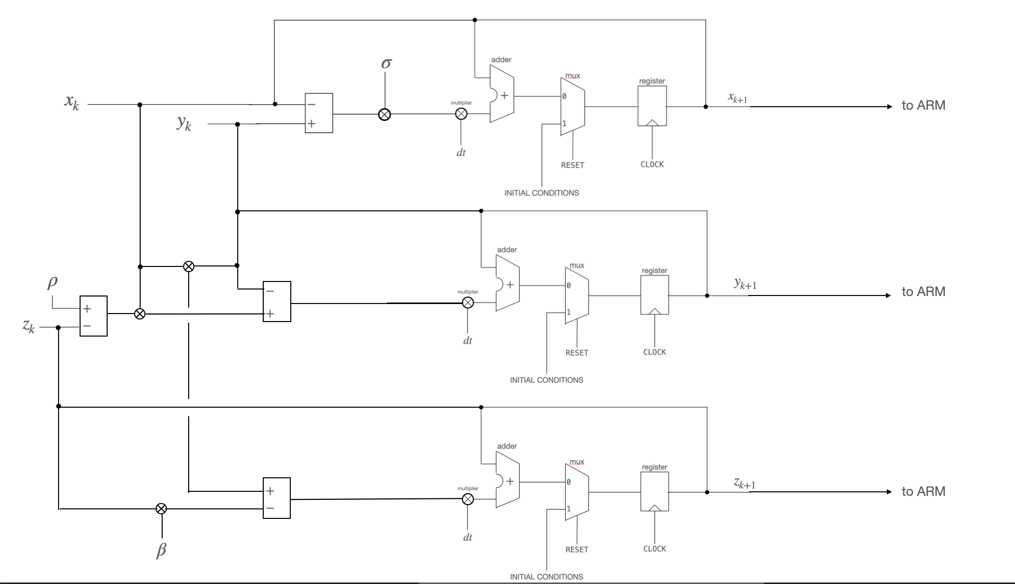
You will be asked to implement the above Euler integrator in hardware using Verilog. The circuit that you will build is illustrated below.
Setup and resources
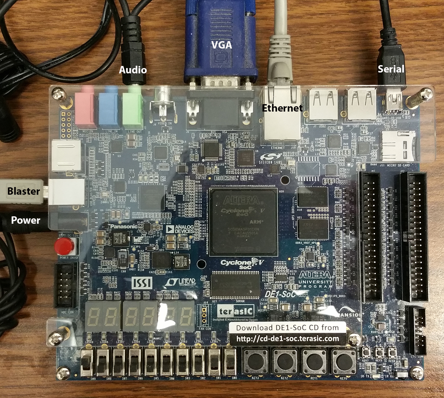
For most exercises there will be 5 or six connections to the board: serial, ethernet, VGA, audio (for lab 2), USB blaster, power. See the image below.
You will find the following resources useful:
Procedure and Weekly Checkpoints
Week 0
- Use this guide to get the DE1-SoC setup.
- Read the policy page!
- Review Verilog basics.
- Review Direct Digital Synthesis.
- Get the DDS demonstration from the ModelSim page running, and add a second sine-wave output which is 90 degrees out of phase with the first.
Week 1
- Read the DDA webpage. After reading the page down through Second order system, stop. The integrator code that you want to start from is in this snippet.
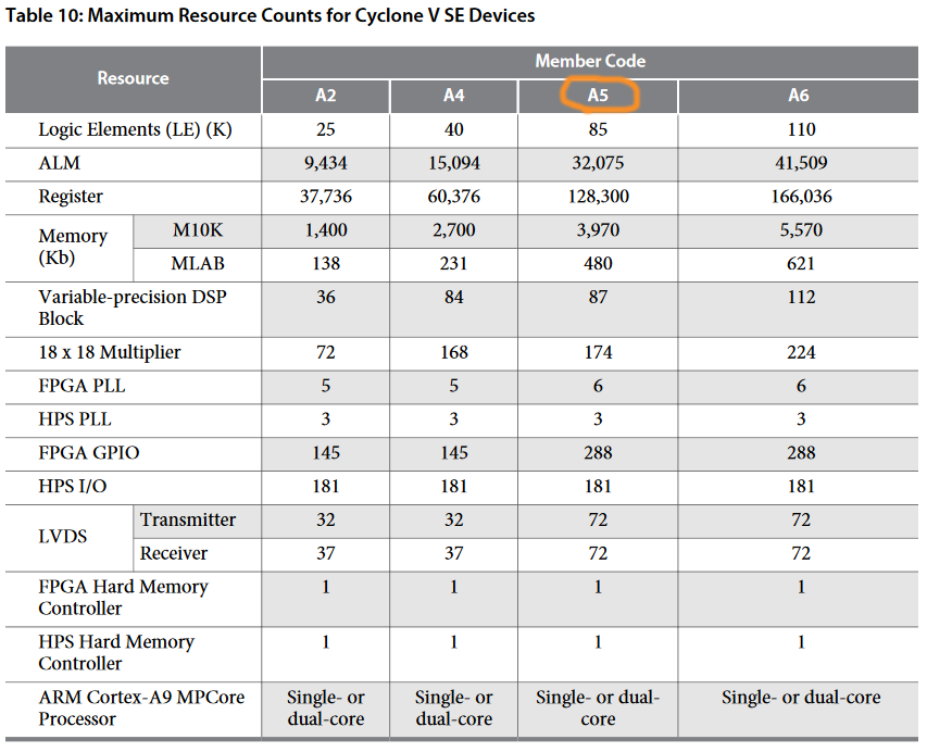
- Read about fixed point arithmetic. We suggest a fixed point format of something like 7.20, with a range of +/-63 and a delta of 10−6. You will need to use a signed, fixed-point multiplier module and an integrator module similar to those in this code snippet. The arithmetic system will use 27-bit multiplies, which on our FPGAs take one hardware multiplier (DSP module). You could use floating point (and Floating DDA) instead, if you want to be slightly adventurous.
- Start by simulating in Matlab or Python! On the FPGA you are going to be using a simple Euler integration. The Python program above is coded to use Euler integration so that you can directly compare the FPGA solution. Make sure that for the constants and initial conditions that you choose no state variable (or intermediate result) goes outside the range +/-63.
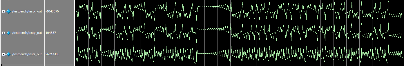
- Next, simulate your synthesizable verilog in Modelsim until you get the same result as you did in Matlab or Python. You will need to write a testbench which sets the same constants and initial conditions as the Python code. One way to check the solver is to export the Modelsim solution vectors to Matlab or Python and create a 3D plot similar to this one. Your Modelsim traces will look something like those shown below.
- Get the Audio Output Bus Master example from the Quartus 18.1 webpage running, and demonstrate a tone being generated from the speakers. You do not need to modify this example at all this week, just load it onto the FPGA and run it. Read about the Altera audio core!
- Once you've verified your compute module in Modelsim (not before!), you're ready to read the solutions back to the HPS for visualization on the VGA display.
Week 2
- Test 2D drawing from the HPS to the VGA display by drawing a sine wave data plot. A good place to start for the HPS to VGA interface is to search for Video VGA 640x480 displayed from SDRAM, in 16-bit color on the Quartus 18.1 example page. In particular, start from the final example in that section (the graphics primitives in 16-bit color example).
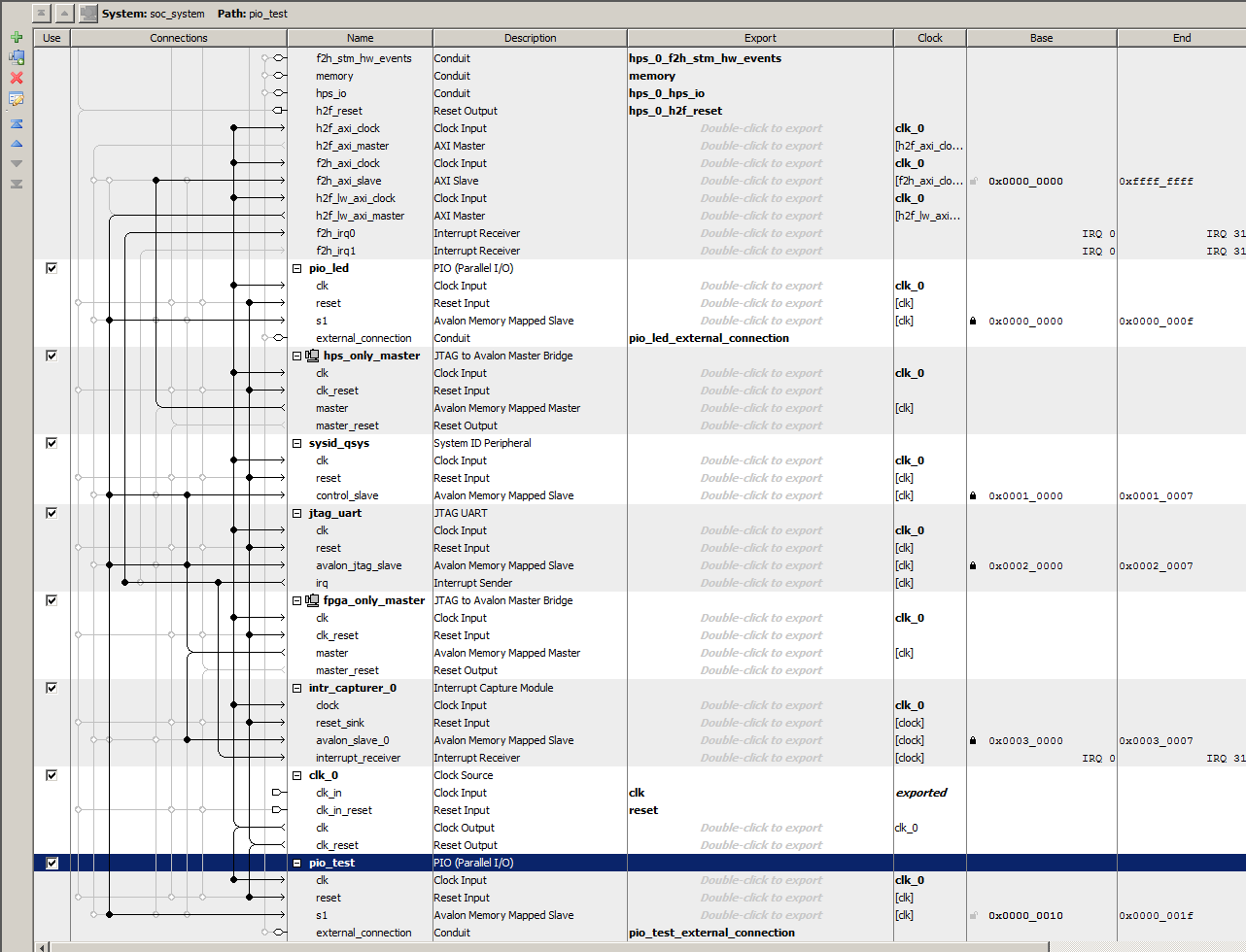
- Connect your solver output to the HPS using parallel i/o port bus-slaves. In Qsys, remember to export the connections to the FPGA solver. Also remember that you have to assign unique addresses in Qsys to each PIO port and use those addresses in the C-code running on the HPS. A small example defines two PIO ports in Qsys, displays counts on LEDs in Verilog, and controls the counts in C. Remember that you will have to sign-extend the 7.20 numbers into full 32-bit notation. The easiest way to do this is to use hardware to concantenate 5 sign bits onto the 27 bit fixed point numbers.
- Demonstrate SignalTap, an onboard logic analyzer, connected to your solver. Prove that the output of your solver on the FPGA matches the output of your solver on Modelsim. Later labs will assume you know how to use SignalTap.

Solver output from Modelsim 
Solver output from SignalTap - Integrate the pure tone synthesizer from the Audio Output Bus Master example on the Quartus 18.1 webpage. The synthesizer need not be connected to the integrator, it can just generate pure tones as before. This will require adding the Audio Subsystem to the Qsys bus, and moving the audio bus master state machine into your code.
- With hard-coded parameter values, demonstrate the hardware solver communicating solutions to the HPS and plotting those solutions to the VGA display. At reset, the system should start drawing all three projections of the Lorenz curve. At this point, you need not have any command-line interface implemented for interacting with this system.
Week 3
- When a hard-coded version plots correctly, build the PIO bus-slaves necessary to control reset function and set constants from the HPS, then start on the command software for console control. I suggest a simple command interpreter to enter the three constants, three initial conditions, start/stop, and reset. You will probably also signal a solution time step request from the HPS to synchronize the solver and the graphics.
- Remember that a parallel I/O port (PIO) which provides data from the HPS to the FPGA is an output! To get the PIO datasheet in Qsys, right-click the module name and in the pop-up menu, select
details>datasheet. Some other modules require that you follow the pathdetails>open_component_folderto get the datasheet. - Add two additional DDS synthesizers, and use the lookup table below to set the dds increment value as a function of the x, y, and z state values. The lookup table takes a 6-bit address between 0 and 51, and returns a 32-bit DDS increment. If necessary, add a constant to any state variable that assumes values that are less than zero, then set the address for the lookup table to bits [25:20] of the resulting 7.20 fixed-point value.
module freq_LUT (
    input wire [5:0] address,
    output wire [31:0] dds_increment_out
) ;
reg [31:0] dds_increment ;
always@(address)
begin
    case(address)
        6'd0: dds_increment=32'd2460658;
        6'd1: dds_increment=32'd2762200;
        6'd2: dds_increment=32'd2925946;
        6'd3: dds_increment=32'd3284755;
        6'd4: dds_increment=32'd3686513;
        6'd5: dds_increment=32'd3905735;
        6'd6: dds_increment=32'd4384445;
        6'd7: dds_increment=32'd4921316;
        6'd8: dds_increment=32'd5524401;
        6'd9: dds_increment=32'd5852787;
        6'd10: dds_increment=32'd6569510;
        6'd11: dds_increment=32'd7373921;
        6'd12: dds_increment=32'd7812366;
        6'd13: dds_increment=32'd8768891;
        6'd14: dds_increment=32'd9842633;
        6'd15: dds_increment=32'd11047908;
        6'd16: dds_increment=32'd11704680;
        6'd17: dds_increment=32'd13138126;
        6'd18: dds_increment=32'd14746949;
        6'd19: dds_increment=32'd15623838;
        6'd20: dds_increment=32'd17537783;
        6'd21: dds_increment=32'd19685266;
        6'd22: dds_increment=32'd22095817;
        6'd23: dds_increment=32'd23410256;
        6'd24: dds_increment=32'd26276252;
        6'd25: dds_increment=32'd29494793;
        6'd26: dds_increment=32'd31248571;
        6'd27: dds_increment=32'd35075566;
        6'd28: dds_increment=32'd39370533;
        6'd29: dds_increment=32'd44191634;
        6'd30: dds_increment=32'd46819617;
        6'd31: dds_increment=32'd52553398;
        6'd32: dds_increment=32'd58988691;
        6'd33: dds_increment=32'd62497142;
        6'd34: dds_increment=32'd70150237;
        6'd35: dds_increment=32'd78741067;
        6'd36: dds_increment=32'd88384163;
        6'd37: dds_increment=32'd93639234;
        6'd38: dds_increment=32'd105106797;
        6'd39: dds_increment=32'd117978277;
        6'd40: dds_increment=32'd124993390;
        6'd41: dds_increment=32'd140300475;
        6'd42: dds_increment=32'd157482134;
        6'd43: dds_increment=32'd176767432;
        6'd44: dds_increment=32'd187278469;
        6'd45: dds_increment=32'd210213595;
        6'd46: dds_increment=32'd235956555;
        6'd47: dds_increment=32'd249987676;
        6'd48: dds_increment=32'd280600950;
        6'd49: dds_increment=32'd314964268;
        6'd50: dds_increment=32'd353535759;
        6'd51: dds_increment=32'd374557834;
        default dds_increment =32'd0 ;
    endcase
end
assign dds_increment_out = dds_increment ;
endmodule
- In your demonstration, you will be asked to set initial conditions/parameter values and then start the integration animation. As the system is animating, we will ask you to speed up/slow down that animation and to pause/resume animation. We will also ask for you to clear the screen while the animation is running. You will be asked to change values for the parameters σ, β, and ρ while the animation is running, and you will be asked to reset the system with a new set of initial conditions. The VGA screen should also display the values for the parameters σ, β, and ρ. All the while, the DDS synthesizers should be generating tones through the speaker so that we can hear the system. The video demonstration at the top of this webpage demonstrates all of the functionality that you will be asked to demonstrate.
Lab reports
Your lab reports should include:
- Everything from the policy page
- Mathematical considerations (type of integrator, error expected/measured, approximations)
- a 3D plot of the solution vectors exported from the Verilog simulator
- Photos of the VGA
- How you implemented the DDA circuits
- A heavily commented listing of your Verilog design and GCC code.